Deriving Latent Dirichlet Allocation using Mean-Field Variational Approach

I haven't yet found a Web tutorial detailing how to derive the formulas for Latent Dirichlet Allocation using a Mean-Field Variational approach, so I thought I could just as well write this blog about it.

Latent Dirichlet Allocation (LDA) is a common technique to determine the most likely topics that are latent in a collection of documents. Blei's (2003) seminal paper introduces LDA and explains a variational approach which is the reference of later work. All tutorials that I have found so far end up referring to Blei's paper, but for people like me, they do not give enough detail.

Wikipedia has a page that explains LDA and how to implement it using Gibbs sampling methods. There's another page in Wikipedia that explains Variational Bayesian methods of the sort that I'm going to cover here, but their examples (based on chapter 10 of  the excellent book by Bishop) do not cover the case of LDA.

So, in this blog I will derive the formulas for the variational approach to LDA from scratch, by relying on the theory and examples explained in Bishop's book.

Generative Model

LDA models a document as being generated from a mixture of topics according to this generative model:

1. For k = 1 .. $K$:
1. $\varphi_k \sim \hbox{Dirichlet}_V(\beta)$ 
2. For m = 1 .. $M$:
1. $\theta_m \sim \hbox{Dirichlet}_K(\alpha)$
2. For n = 1 .. $N_m$:
1. $z_{mn} \sim \hbox{Multinomial}_K(\theta_m)$
2. $w_{mn} \sim \hbox{Multinomial}_V(\sum_{i=1}^KZ_{mni}\varphi_i)$

In this notation, $z_{mn}$ is a vector with $K$ components such that only one of them has a value of 1, and the rest is zero. Similarly with $w_{mn}$. $K$ is the number of topics, $V$ is the vocabulary, $M$ is the number of documents, and $N_m$ is the number of words in document $m$.

The generative process can be expressed with this plate diagram:

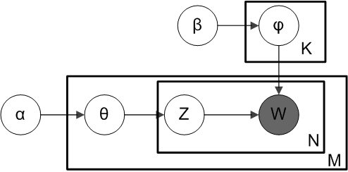
("Smoothed LDA" by Slxu. public - Own work. Licensed under CC BY-SA 3.0 via Wikimedia Common)

Joint Probability

According to the plate diagram the joint probability is:
$$
P(W,Z,\theta,\varphi;\alpha,\beta) = \prod_{k=1}^KP(\varphi_k;\beta)\prod_{m=1}^MP(\theta_m;\alpha)\prod_{n=1}^NP(z_{mn}|\theta_m)P(w_{mn}|z_{mn},\varphi)
$$

If we substitute the probabilities by the respective formulas for the Multinomial and Dirichlet distributions, we obtain:

$$
P(W,Z,\theta,\varphi;\alpha,\beta)= \prod_{k=1}^K(\frac{1}{B(\beta)}\prod_{v=1}^V\varphi_{kv}^{\beta-1}) \prod_{m=1}^M\left(\frac{1}{B(\alpha)}\prod_{k=1}^K\theta_{mk}^{\alpha-1}\prod_{n=1}^N(\prod_{k=1}^K\theta_{mk}^{z_{mnk}} \prod_{k=1}^K\prod_{v=1}^V\varphi_{kv}^{w_{mnv}z_{mnk}} )\right)
$$

Variational Inference

We want to determine the values of the latent variables $\varphi,\theta,Z$ that maximise the posterior probability $P(\theta,\varphi,Z|W;\alpha,\beta)$. According to Bishop, Chapter 10, we can approximate the posterior with a product that separates $z$ and $\theta,\varphi$:
$$
P(\theta,\varphi,Z|W;\alpha,\beta) \approx q_1(Z)q_2(\theta,\varphi)
$$

Here $q_1$ and $q_2$ are families of functions, and we choose $q_1^*$ and $q_2^*$ that best approximate P by applying the formulas:
$$
\ln q_1^* (Z) = \mathbb{E}_{\theta\varphi}\left[\ln P(W,Z,\theta,\varphi;\alpha,\beta)\right] + const
$$
$$
\ln q_2^* (\theta,\varphi) = \mathbb{E}_{Z}\left[\ln P(W,Z,\theta,\varphi;\alpha,\beta)\right] + const
$$

The constants are not important since we can determine their exact values later. Also, since these formulas use logarithms, the calculations can be simplified as we will see below.

 

Factor with $Z$

Let's start with $q_1(Z)$:

$$\ln q_1^*(Z) = \mathbb{E}_{\theta\varphi}\left[\ln P(W,Z,\theta,\varphi;\alpha,\beta)\right] + const$$

$$ = \sum_{k=1}^K\left((\beta-1)\sum_{v=1}^V\mathbb{E}(\ln\varphi_{kv})\right) $$

$$+ \sum_{m=1}^M\left((\alpha-1)\sum_{k=1}^K\mathbb{E}(\ln\theta_{mk})+\sum_{n=1}^N\left(\sum_{k=1}^Kz_{mnk}\mathbb{E}(\ln\theta_{mk})+\sum_{k=1}^K\sum_{v=1}^Vz_{mnk}w_{mnv}\mathbb{E}(\ln\varphi_{kv})\right)\right)+const$$

In this expression, terms that do not contain the variable $z$ are constant and therefore can be absorbed by the general $const$, simplifying the expression:

$$=\sum_{m=1}^M\sum_{n=1}^N\left(\sum_{k=1}^Kz_{mnk}\mathbb{E}(\ln\theta_{mk})+\sum_{k=1}^K\sum_{v=1}^Vz_{mnk}w_{mnv}\mathbb{E}(\ln\varphi_{kv})\right)+const$$
$$=\sum_{m=1}^M\sum_{n=1}^N\sum_{k=1}^Kz_{mnk}\left(\mathbb{E}(\ln\theta_{mk})+\sum_{v=1}^Vw_{mnv}\mathbb{E}(\ln\varphi_{kv})\right)+const$$

We can observe that the expression can be reduced to a combination of probabilities from multinomial distributions, since $\ln\left(\hbox{Multinomial}_K(x|p)\right) = \sum_{i=1}^Kx_i\ln(p_i)+const$ and conclude that:

$$q_1^*(Z)\propto\prod_{m=1}^M\prod_{n=1}^N\hbox{Multinomial}_K\left(z_{mn}\middle|\exp\left(\mathbb{E}(\ln\theta_m)+\sum_{v=1}^Vw_{mnv}\mathbb{E}(\ln\varphi_{.v})\right)\right)$$

We can determine $\mathbb{E}(\ln\theta_m)$ and $\mathbb{E}(\ln\varphi_{.v})$ if we can solve $q_2(\theta,\varphi)$ (see below).

Factor with $\theta,\varphi$

$$\ln q_2^* (\theta,\varphi) = \mathbb{E}_{Z}\left[\ln P(W,Z,\theta,\varphi;\alpha,\beta)\right] + const$$

$$=\sum_{k=1}^K\left((\beta-1)\sum_{v=1}^V\ln\varphi_{kv}\right) $$

$$+ \sum_{m=1}^M\left((\alpha-1)\sum_{k=1}^K\ln\theta_{mk}+\sum_{n=1}^N\left(\sum_{k=1}^K\mathbb{E}(z_{mnk})\ln\theta_{mk}+\sum_{k=1}^K\sum_{v=1}^V\mathbb{E}(z_{mnk})w_{mnv}\ln\varphi_{kv}\right)\right)+const$$

All terms contain $\theta$ or $\varphi$ so we cannot simplify this expression further. But we can split the sum of terms into a sum of probabilities of Dirichlet distributions, since $\ln(\hbox{Dirichlet}_K(x|\alpha))=\sum_{i=1}^K(\alpha_i-1)\ln(x_i) + const$:

$$=\left(\sum_{k=1}^K\left((\beta-1)\sum_{v=1}^V\ln\varphi_{kv}\right)+\sum_{m=1}^M\sum_{n=1}^N\sum_{k=1}^K\sum_{v=1}^V\mathbb{E}(z_{mnk})w_{mnv}\ln\varphi_{kv}\right)$$

$$+\left(\sum_{m=1}^M\left((\alpha-1)\sum_{k=1}^K\ln\theta_{mk}+\sum_{n=1}^N\sum_{k=1}^K\mathbb{E}(z_{mnk})\ln\theta_{mk}\right)\right) + const$$

$$= (1) + (2) + const$$

Note that $(1)$ groups all terms that use $\varphi$, and $(2)$ groups all terms that use $\theta$. This, in fact, means that $q_2(\theta,\varphi)=q_3(\theta)q_4(\varphi)$, which simplifies our calculations. So, let's complete the calculations:

Subfactor with $\varphi$

$$\ln q_4^*(\varphi) = $$

$$= \sum_{k=1}^K\left((\beta-1)\sum_{v=1}^V\ln\varphi_{kv}\right)+\sum_{m=1}^M\sum_{n=1}^N\sum_{k=1}^K\sum_{v=1}^V\mathbb{E}(z_{mnk})w_{mnv}\ln\varphi_{kv}+ const$$

$$= \sum_{k=1}^K\sum_{v=1}^V\left(\beta -1 +\sum_{m=1}^M\sum_{n=1}^N\mathbb{E}(z_{mnk})w_{mnv}\right)\ln\varphi_{kv} + const$$

Therefore: $q_{4}^*(\varphi) \propto \prod_{k=1}^K\hbox{Dirichlet}_V\left(\varphi_k\middle|\beta+\sum_{m=1}^M\sum_{n=1}^N\mathbb{E}(z_{mnk})w_{mn.}\right)$

Subfactor with $\theta$

Similarly, $\ln q_3^*(\theta) = $

$$\sum_{m=1}^M\left((\alpha-1)\sum_{k=1}^K\ln\theta_{mk}+\sum_{n=1}^N\sum_{k=1}^K\mathbb{E}(z_{mnk})\ln\theta_{mk}\right) + const$$

$$ = \sum_{m=1}^M\sum_{k=1}^K\left(\alpha-1 + \sum_{n=1}^N\mathbb{E}(z_{mnk})\right)\ln\theta_{mk} + const$$

Therefore: $q_{3}^*(\theta) \propto \prod_{m=1}^M\hbox{Dirichlet}_K\left(\theta_m\middle|\alpha+\sum_{n=1}^N\mathbb{E}(z_{mn.})\right)$

Algorithm

Now we can fit all pieces together. To compute $q_1^*(Z)$ we need to know $q_3^*(\theta)$ and $q_4^*(\varphi)$, but to compute these we need to know $q_1^*(Z)$. We know that $q_1^*(Z)$ follows a Multinomial distribution, and $q_3^*(\theta)$ and $q_4^*(\varphi)$ follow Dirichlet distributions, so we can use their parameters to determine the expectations that we need:

• From the properties of Multinomial distributions we know that $\mathbb{E}(z_{mnk}) = p_{z_{mnk}}$, where $p_{z_{mnk}}$ is the Multinomial parameter. Therefore we can conclude that:
• $q_3^*(\theta) \propto \prod_{m=1}^M\hbox{Dirichlet}_K\left(\theta_m\middle|\alpha+\sum_{n=1}^Np_{z_{mn.}}\right)$
• $q_4^*(\varphi) \propto \prod_{k=1}^K\hbox{Dirichlet}_V\left(\varphi_k\middle|\beta+\sum_{m=1}^M\sum_{n=1}^Np_{z_{mnk}}w_{mn.}\right)$
• From the properties of Dirichlet distributions we know that $\mathbb{E}(\ln\theta_{mk}) = \psi(\alpha_{\theta_{mk}}) - \psi\left(\sum_{k'=1}^K\alpha_{\theta_{mk'}}\right)$, where $\alpha_{\theta_{mk}}$ is the Dirichlet parameter and $\psi(x)$ is the digamma function, which is typically available in standard libraries of statistical programming environments. Therefore we can conclude that:
• $q_1^*(Z) \propto \prod_{m=1}^M\prod_{n=1}^N\hbox{Multinomial}_K\left(z_{mn}\middle|\exp\left(\psi(\alpha_{\theta_{m.}}) - \psi\left(\sum_{k'=1}^K\alpha_{\theta_{mk'}}\right) + \sum_{v=1}^Vw_{mnv}\left(\psi(\beta_{\varphi_{.v}})-\psi\left(\sum_{k'=1}^K\beta_{\varphi_{k'v}}\right)\right)\right)\right)$

We are now in the position to specify an algorithm that, given some initial values of one of the parametres, it calculates the other, then it re-calculates the parametres alternatively until the values do not change beyond a threshold. The algorithm is:

1. For m=1..M, n=1..N, k=1..K
1. $p_{z_{mnk}}=1/K$
2. Repeat
1. For k=1..K, v=1..V
1. $\beta_{\varphi_{kv}}=\beta+\sum_{m=1}^M\sum_{n=1}^Nw_{mnv}p_{z_{mnk}}$
2. For m=1..M, k=1..K
1. $\alpha_{\theta_{mk}}=\alpha+\sum_{n=1}^Np_{z_{mnk}}$
3. For m=1..M, n=1..N, k=1..K
1. $p_{z_{mnk}}=\exp\left(\psi(\alpha_{\theta_{mk}}) - \psi\left(\sum_{k'=1}^K\alpha_{\theta_{mk'}}\right) + \sum_{v=1}^Vw_{mnv}\left(\psi(\beta_{\varphi_{kv}})-\psi\left(\sum_{k'=1}^K\beta_{\varphi_{k'v}}\right)\right)\right)$

Note that step 2.1.1 means that $\beta_{\varphi_{kv}}$ is an update of $\beta$ with the expected number of times that word $v$ is assigned topic $k$. Likewise, step 2.2.1 means that $\alpha_{\theta_{mk}}$ is an update of $\alpha$ with the expected number of words in document $m$ that are assigned topic $k$. Finally, $p_{z_{mnk}}$ is the probability that a word in place $n$ of document $m$ is assigned topic $k$.

Some additional notes about this algorithm:

1. The initialisation step just assigns $1/K$ to each element of $p_z$, but note that Bishop said that there are several local minima. Different initial states may lead to different results. So it may be worth to research the impact of initial values in the final result.
2. There are several iterations over the entire vocabulary $V$, which may be computationally-expensive for large vocabularies. We can optimise this by noting that $w_{mn}$ is a vector of $V$ elements such that only one of them has a value of 1, and the rest is zero.
3. Steps 1 and 2 inside the repeat cannot be done in parallel with step 3, but all steps inside these can be made in parallel, so this is an obvious place where we can use GPUs or CPU clusters. 

So this is it. The final algorithm looks different from the original algorithm from Blei's paper, so I'm keen to hear any comments about whether they are equivalent, or whether there are any mistakes in the derivation.

Code

I implemented the algorithm in a Python program, but for some reason I do not get the expected results. I suspect that the step that derives $\theta$ and $\varphi$ from $\alpha_{\theta_{mk}}$, $\beta_{\varphi_{kv}}$ and $p_{z_{mnk}}$ is wrong, but there might be other mistakes.

The code is in http://github.com/dmollaaliod/varlda

If you can find out what is wrong, please post a comment, or drop me a message.

Scubawatch - A pebble app for scuba divers

Did you know that the original pebble smartwatch is waterproof to 50 metres? Well I tested it in my recent dives. I took it down to 28 metres, and it still works without problems. So, I created an app that can help me track my air consumption during my dives.

The app is very simple. When it starts, a timer will show the duration of the dive. You can use the up and down buttons to change the display of air pressure in bar, and the new value will be recorded in a log after a delay of 3 seconds.

To view the log, do a long press on the select button. To reset the time and the log, double-press on the select button, or simply exit the app.

Currently the app is very simple, and the log keeps only the last 10 records.

You can find the app in the pebble app store. If you want to improve it, check the code at: https://github.com/dmollaaliod/scubawatch

Here are a couple of screenshots [Update: the screenshots show the new version that also incorporates compass heading]. I haven't taken it under water yet. Let me know if you find it useful!

I haven't made this version available for the new pebble time series because they can be taken only to 30 metres. So, I may buy a few of the old models. They are much cheaper, and probably more useful for scuba divers.

Including mathematical expressions in blogger

Yesterday I spent some time trying to figure out how to include mathematical expressions in blogger. All the solutions that I saw consist of inserting a piece of JavaScript code in the blog template or plugins list. This JavaScript processes LaTeX expressions and renders them in blogger.

After quite a while I managed to make the system work. I used MathJax as the LaTeX rendering machine, and I basically followed the procedure listed here:

• How to Enable LaTeX Equations in Blogger using MathJax
• How to Write Math or Equation on Blogger/Blogspot (UTube video)

I didn't follow exactly what these links do. The first one wasn't very clear, and I didn't manage to make the system work. The second is a video that says more than what you need, especially if you already know how to write LaTeX mathematical expressions. This is what I did:

1.  At the dashboard, select the blog that you want to use, and then select "Templates" on the menu at the left-hand side.
2. Select a basic template, not a dynamic template (according to a comment by Sobresaliente to the first link, it doesn't work if you use dynamic templates).
3. Click "Edit HTML".
4. Click the box "Expand Widget Templates" (I didn't this in a previous attempt and it didn't work, so make sure that you click on that box!).
5. Insert the following text at the end of the head section. Insert it at the end, not at the beginning!

That's all. To insert an inline equation, simply enclose the equation between dollar symbols, and to insert an equation centered on the page, enclose it between double dollar symbols. I still need to figure out how to type a dollar symbol without triggering the conversion to LaTeX formulas!

Now I can pretend to be as smart as Einstein and claim that $e=mc^2$. Or, if you want to see one of my posts using mathematical formulas, look at this one:

• Implementation of Gibbs sampling for Naive Bayes text classification

Since I tried different methods I'm not sure if the above steps will work for everybody, I may have missed something... so if you try it, post your experience here!

Implementation of Gibbs sampling for Naive Bayes text classification

This post is related to the Gibbs sampling implementation described by Resnik & Hardisty (2010), Gibbs sampling for the uninitiated, CS-TR-4956. The referred paper is a very good tutorial on Gibbs sampling, and they work through an example of Gibbs sampling for text classification using "Naive" Bayes. I add quotation marks because the approach presented is slightly more informed than the traditional Naive Bayes method.

In the traditional Naive Bayes method, the idea is that, given a document $j$, the task is to find the label $L_j$ that maximises the probability $P(L_j|W_j)$, where $W_j$ is a vector of features. This approach uses the Bayes rule, and as a result the problem is transformed to one of finding the label that maximises:

$$
P(L_j|W_j) = \frac{P(W_j|L_j) P(L_j)}{P(W_j)}
$$


Since $P(W_j)$ is constant in the document $j$, we can ignore the denominator. The prior $P(L_j)$ is estimated by counting the number of times label $L_j$ is assigned to a document in the training data, and dividing by the number of training documents.

To compute $P(W_j|L_j)$ we introduce the naive assumption that all features are independent of each other, and therefore $P(W_j|L_j)$ is the product of all $P(W_{ji}|L_i)$, for each $W_{ji}$ separate feature value. Each individual $P(W_{ji}|L_i)$ can then be estimated using the maximum likelihood estimate on the training data, that is, by counting.

Okay, that's the known Naive Bayes method. Resnik & Hardisty's method simulates this Naive Bayes approach for text classification by offering this generative story of the documents to classify:

1. The label $L_j$ of a given document is randomly generated by flipping a coin with heads probability $\pi = P(L_j=1)$. In other words and more formally, $L_j$ is sampled from a Bernoulli distribution with probability $\pi$.
2. Words in the document $j$ are generated randomly and independently of each other, according to a probability that depends on the chosen $L_j =0$ or $L_j = 1$. This is simulated by throwing a multi-faceted die with as many faces as different words. We throw the die once per word we want to generate. The feature $W_{ji}$ indicates the number of times a word $i$ has been obtained. In other words and more formally, $W_{ji}$ is sampled from a Multinomial distribution with probability distribution theta depending on the value of $L_j$.

Note that step 2 is a little more informed than in a generic Naive Bayes approach, since we are saying that a feature $W_{ij}$ is not drawn from some unknown distribution. It is a Multinomial distribution and this fact is exploited by Resnik & Hardisty.

Given this generative story, the joint distribution of all document word frequencies $W$, labels $L$, label probability $\pi$, and word distributions $\theta_0$ and $\theta_1$ are computed as described in the paper (I won't go into this here). After some simplifications, the task is handed over to the Gibbs sampler, which is used to estimate the values of this joint distribution in the manner that is explained in the paper so well. Basically, the idea of the Gibbs sampler is to sample a new value of a parameter by removing this parameter, computing the probability of this parameter given the other parameters, and sampling a new value of the parameter. This is done with all parameters a number of times until we think we have reached a good value... more about this later. The final algorithm looks like this:

At every iteration, given the counts previously computed of all words and documents associated to a label class:

1. For every document $j$:
   If $j$ is not a training document then:
   
   • Subtract $j$'s word counts from the total word counts associated to label class $L_j$
   • Subtract $1$ from the count of documents with label $L_j$
   • Assign a new label $L_j$ as described in the paper
   • Add $1$ to the count of documents with label $L_j$ (note that $L_j$ may be different now)
   • Add $j$'s word counts to the total word counts associated to label class $L_j$
2. Sample new values of $\theta_0$ given word counts associated to label $0$
3. Sample new values of $\theta_1$ given word counts associated to label $1$

Due to practical reasons I had to do a simple modification. This modification is due to the problem of computing the new label $L_j$, which involves computing a product of theta values raised to the power of word counts. This computation can easily produce numbers very close to zero which may overwhelm the representation ability of the computer (underflow). So I used logarithmic values and changed products to sums, and exponents to multiplications. Then, since the final operation in the computation involved a division, I simply subtracted values and then obtained the final value by raising $e$ to the power of our number.

I tried the program with artificial documents generated exactly as described in the generative model, and I was pleased to see how well it was able to predict the labels given very few samples.

I also noticed that only two to three iterations were usually required to obtain stable values of $L_j$ (though the values of theta were not stable at that moment). The following figure represents the histograms of 10 distributions. Each distribution uses 1000 document sets randomly generated and then partitioned into a training and a test set. Each set contains 50 documents of 100 samples from a multinomial with 5 distinct words, and the Gibbs sampling used 5 iterations. I chose the labels of the last iteration (instead of the mode of the last three iterations, which is probably wiser). Each plot represents a distribution where the ratio between training and test set differs. We can appreciate how quickly the system learns:

Note that, for a ratio of 0, the system does not use any training set and therefore the process is completely unsupervised. We appreciate a symmetric distribution due to inversions between 0 and 1 in half of the cases. So, really, the accuracy of the unsupervised process, as we view it as a case of clustering, should be doubled. As we increase the percentage of training documents, the system has more information to avoid inversion. I actually found it surprising that we need up to 50% of the documents for training to get rid of the zeros, I expected we would need only a handful of documents.

But we can really see that this approach is very effective with very few documents. Of course the figure is based on an ideal case when the documents are generated exactly as per the generative model. The next step would be to test the robustness of the model against real-world documents, i.e., against documents that do not follow the generative model.

The implementation is available in http://sourceforge.net/p/nbgibbs. Feel free to download and use the code, and give feedback here or in the sourceforge page.

Problems with the video drivers in Ubuntu 11.04

Last Friday I upgraded my desktop to Ubuntu 11.04, and yesterday Saturday I upgraded my laptop. In both cases I had problems with the video drivers and I think I solved them. Just in case someone is having similar problems, here I'll write about the problems I had and what I did to solve them. I'm writing this from memory so I may have missed some of the many things I tried, or I did them in the wrong order, or in the writing I mix up the exact names of the software I used and the options I selected... but hopefully this information is still useful.

My desktop computer has dual monitor and an nvidia graphics card. I didn't manage to make the nvidia drivers work with the previous release so I was using the default drivers, which worked well enough for me since I didn't use the computer for fancy graphics or games. But when I upgraded to Ubuntu 11.04 I had problems with the display.

On the first startup, the monitors froze after logging in. I could only see the desktop background, that's all. There were no menus, no mouse pointer, nothing. Just the background image. I restarted a couple of times in ubuntu and in the other OS, Windows 7, but whenever I logged into Ubuntu I could only see the background image.

The first thing I did was to load the recovery version, and select the option to repair broken packages. The system didn't report anything special: no packages were found broken, so nothing was done. And again, after logging in, I could only see the background image.

Next I tried to login in with the failsafe display. Login was successful but the display behaved in a very strange manner. The monitor on the left had a black screen and the mouse pointer, whereas the monitor on the right had the desktop contents. To click on an item on the monitor on the right I had to use the mouse on the monitor on the left and predict where I was clicking... a very strange setup and very frustrating!

So I disconnected one monitor and restarted again. Now mouse and desktop were in the one monitor but there were no window decorations so I could not move or resize the windows. And it wasn't displaying the new "unity" desktop graphics but the classic one.

I tried several options. First of all I logged in again, this time asking to re-configure the graphic display (this is an option I saw when logging in on the failsafe session), but again the windows had no decorations and the desktop had the classic setup instead of the "unity" setup.

Finally I asked to use the generic display when logging in with the failsafe session and I managed to have the "unity" graphics. I asked to have the new graphic setting permanent, plugged the second monitor, and logged in again. The "unity" graphics appeared the contents of the two monitors were replicated. I opened the monitor manager and I selected the "extended desktop" option. Now everything was displayed as I wanted! I was so excited to see it apparently working and I was so late for dinner that I went home without checking whether the windows had decorations... I'll find out tomorrow Monday.

Yesterday Saturday I upgraded the laptop. During the upgrade the system reported errors with the xorg package so expected the worse. And true, after restarting the system would not even show the login page. Instead, the monitor showed a mix of colourful pixels.

The first thing I did was to select the option to repair broken packages in the recovery session, and to my relief it reported that some packages were repaired. Yet after restarting the monitor still showed the mix of colourful pixels in apparent random distribution. Next I selected the option to reconfigure the graphics but again, nothing interesting happened.

Next I selected the option to use the generic display, and now I could log in and see the desktop. Success! The windows had decorations, but the desktop setup was the classic, not the "unity" setup, because a message said that the laptop didn't have the hardware to run unity. I couldn't believe that since the laptop has an nvidia card which is supposed to be powerful enough. I opened the "restricted drivers" interface but it didn't show the nvidia driver there. I searched in synaptics package manager and I found several drivers, but they could not be installed because the source was not enabled. So I enabled the source and opened the "restricted drivers" interface. Now I could see the recommended nvidia drivers there, great! I selected the recommended one, and after re-starting I could see the unity interface.

Success! now I can use the laptop, and hopefully the desktop at my office works too.

The next thing is to get used to the unity interface. So far it doesn't look as useful as the classic one so I may end up switching to the classic one but let's give it a few more days.

How to install a Python module in Windows?

The Python documentation is very detailed on how to install Python modules: you simply type something like this at the terminal window:

python setup.py install

The problem is, how do you do this in a Windows-based PC? I tried the following but it didn't work:

1. Open a command prompt by type "cmd" at the "Run..." option from the start menu (I'm using Windows XP)
2. Navigate to the folder where we have downloaded our Python module
3. Type python setup.py install

When I tried that I got this error message:

'python' is not recognized as an internal or external command, operable program or batch file.

The problem is that the path of the executable python.exe is not listed in the PATH environment variable. I went round the problem by typing the exact location of the executable:

C:\python27\python setup.py install

But then I got another error! It turns out that the package I wanted to install requires another package called setuptools... back to the drawing board.

Fortunately I found documentation about setuptools. The module is packaged for a range of distributions including Windows, I only need to run its executable to install the package. And the good thing of this module is that provides a program called easy_install, which is located in C:\Python27\scripts. With this program you can actually install many other packages. It will download the package, install it, and solve any possible dependencies by downloading and installing additional packages.

So, to install a new Python package, say, suds, in a Windows PC, my current sequence of steps was:

1. Open a command prompt as before.
2. Type C:\Python27\scripts\easy_install suds

End of story! and it works! for me, anyway. You can find additional documentation about easy_install here.

How do I setup a Huawei E220 USB wireless modem in Ubuntu linux?

I have one of those USB wireless modems, a Huawei E220, which I can use to access the internet from many Australian cities using the three network. The modem works fine in Windows but I had many problems to make it work in Ubuntu. I finally found some useful information on the web, and the process is not as hard as I thought could be. Here's a summary of how to do it. But first of all, an explanation of how the modem works.

After plugging in the USB modem, two USB devices are created in /dev/TTYusb0 and /dev/ttyUSB1. The first one, /dev/ttyUSB0, is the actual modem. The computer sees the modem as a dial-up modem. So to use it, the computer needs to use the modem and "call" a special phone number via the modem. This can be done with the program wvdial.

To configure wvdial, edit the file /etc/wvdial.conf so that it looks like this (you need to edit with sudo and have administrator permissions):

[Dialer Defaults]
Init1 = ATZ
Init2 = ATQ0 V1 E1 S0=0 &C1 &D2 +FCLASS=0
Modem Type = Analog Modem
ISDN = 0
Modem = /dev/ttyUSB0
Phone = *99#
Username =
Password =
Baud = 460800
New PPPD = yes

That's it! You can type whatever you want as a username and password. Now plug the modem, wait for a few minutes until the device /dev/ttyUSB0 exists, and run the following command:

wvdial Defaults

For some reason that I don't understand, the first time I try this the connection always drops, so I need to unplug the modem, plug it again, wait a few minutes and then type wvdial Defaults again. Then it works.

How do I set a dual screen output for Linux Ubuntu/Kubuntu?

Linux does have many good things, but sometimes you really need to try hard to get the best of it, or even to do what is taken for granted, say, in Windows. One example is for allowing a laptop to use an external monitor. I have a Dell laptop, model XPS M1210 with nVidia graphics card. The laptop has two partitions, one with Windows Vista, and the other with Linux Ubuntu or Kubuntu, both are basically the same thing with different clothes. I use this laptop to give lectures at Macquarie University and therefore the external monitor is essential. But I haven't yet managed to use the external monitor under Ubuntu easily.

Under Windows Vista, you just need to type Fn+F8. This combination of keys alternates the use of the laptop screen, the external screen, or both. However, in Ubuntu you first need to do a lot of under-the-hood tinkering until you get something that works somewhat.

First, I had to install the nVidia driver. Some time ago I unsuccessfully tried to do it, until I found Envy, an installer written by Alberto Milone that does all the job very easily. Thanks so much Alberto! This was last year, when I was using a former version of Ubuntu (was it Feisty Fawn...?). Recently I tried to use it again to re-install the driver but it didn't work any more... pity. There are other options, or so the Synaptic Package Manager tells me. I tried some of them but I don't remember which ones worked and which ones didn't work.

Anyway, once you get the driver installed you need to edit one of those mysterious files, in particular the file /etc/X11/xorg.conf. Before you even think of editing this file it's best if you make a back up of it, otherwise you might not be able to use your graphic display any more. Since you need the superuser privileges you need to type the following:

sudo cp xorg.conf xorg.conf.bkup

Then, edit the file using your favourite editor. Mine is emacs. Since you need to use superuser privileges to edit this file, you edit it by typing:

gksudo emacs xorg.conf

Then you need to specify that the screen uses Twin View, and some characteristics such as screen resolution. This is what I added to the entry Section "Screen":

#    Option         "RenderAccel" "True"
  Option         "TwinView"          
#    Option         "TwinViewOrientation" "Clone"
  Option         "MetaModes" "1280x800,1280x800; 1280x1024,1280x1024; 1024x768,1024x768"
  Option "SecondMonitorHorizSync" "50"
  Option "SecondMonitorVertRefresh" "60"
#    Option "UseDisplayDevice" "DFP, CRT"
#    Option "ConnectedMonitor" "CRT"

Noted that some of the text is commented out? This is because I haven't yet managed to work the way I want, but I'm coming to this in a minute. Just to finish, you need to save the file, plug the external monitor, and then restart the window manager by typing Alt-Ctrl-Backspace. You could also restart the system completely but of course that takes longer.

In theory this should make it work, or at least the tutorials listed below say. But I haven't yet managed to have both the laptop screen and the external monitor active. More often than not, the laptop screen appears completely blank and I can only use the external monitor. I tried to add other options following some suggestions from the Internet, but none of them helped, and in some occasions (such as the options "useDisplayDevice" and "ConnectedMonitor" made things worse.

So well, I can use the external monitor after several hours of trying, but it's not yet the way I wanted it to work... I'll keep trying.

Some tutorials that I used:

• http://www.ubuntugeek.com/dual-monitors-with-nvidia.html
• http://ubuntuforums.org/showthread.php?t=221174
  
• http://http.download.nvidia.com/solaris/1.0-8762/README/appendix-g.html
  

Setting the default display manager in Ubuntu/Kubuntu

One of the good things of Ubuntu, and Linux in general, is that there is a wide range of windows managers. You aren't stuck to the look and feel given by a company, but you can choose among several options. Two of the most popular windows managers in the Linux world are GNOME and KDE. The default manager in Ubuntu is GNOME, but if you use Kubuntu, the default is KDE.

Kubuntu and Ubuntu are very much the same thing but the looks are different, using different user interface philosophies. Ubuntu/GNOME is robust and ideal for those who want to use the computer for productivity, whereas Kubuntu/KDE is flexible and customisable and ideal for those who like looking "under the hood", but it's less reliable (sometimes you really need to look under the hood to fix some specific problems).

I generally find the look and feel of GNOME more elegant, and that of KDE more nerdy, but that's just my opinion.

I sometimes like GNOME, other times prefer KDE, and I end up switching from one to the other whenever one of them announces a new improvement, which is quite often.

But surprisingly I found very little information about how to switch from one to the other... finally, after looking here and there, I found out. It's simple, as these things are once you know them. Here's what you need to do:

• If you are under Ubuntu (GNOME) and want to switch to Kubuntu, simply install kubuntu-desktop by using Synaptics or your favourite package manager
• If you are under Kubuntu (KDE) and want to switch to Ubuntu... well, simply install ubuntu-desktop by using adept_manager or your favourite package manager

KDM and GNOME have their own display managers, and oddly enough KDM does work fine under GNOME's display manager, and vice-versa. So there's no real need to change display managers unless you want to. To do this, after installing kubuntu_desktop or ubuntu_desktop simply edit the file /etc/X11/default-display-manager so that it has the following contents:

• /usr/sbin/gdm to set GDM, that is, the Gnome display manager
• /usr/bin/kdm to set KDM, the KDE display manager
• /usr/lib/kde4/bin/kdm to set KDM for KDE4, the new version of KDE which is still under experimentation. To use KDE4 you will need to install the package kubuntu-kde4-desktop (you guessed right)

I like the look and feel of GNOME but I want the flexibility of many of the programs associated with KDE (such as digikam for managing photos, or amarok for playing music). The good thing is that these programs also run under GNOME so it is actually possible to get the best of both worlds.

I can't delete a KDE4 widget

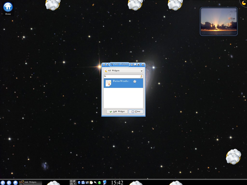
Last week I installed Furius Weather, a cool widget for KDE4 that displays the weather in your preferred location. This widget, though, is not perfectly integrated in the KDE4 plasma, and for example you can't add it to the task bar at the bottom, or at least I didn't manage to do it.

I tried to add it by following the usual procedure: select "Add widgets" on right-click at the desktop, and then drag the entry for Furius weather to the bar. When I did that, a dialogue appeared that prompted for a theme. I selected my default theme which I had downloaded from Furius Weather. To my horror I saw that the default theme uses large icons which did not fit on the task bar.

I tried to delete the widget using the usual way: select "Add widgets" and click on the star next to Furius Weather, but nothing happened. Actually, I don't know how I ended up having three instances in my task bar! See the image. Now I had almost no space for anything else in the bar.

Today, finally I found the solution. You need to edit the file ~/.kde4/share/config/plasma-appletsrc. In the file I found 18 references to FuriusWeather! I guess that was how many times I added the widget and tried to delete it. I removed all references, restarted the window manager (ALT CTRL <-; don't just log out or restart the computer or KDE will overwrite your modifications), and the desktop came back clean.

Wonderful!

How can I add a personalised wallpaper to KDE4?

I have been trying KDE4 for a few months. This is the new version of KDE, a Linux desktop that has a beautiful interface. But currently it's not as easy to customise as the old trusty KDE 3. For example, do you know how to use one of your own photos as a wallpaper? There are no right-click actions on dolphin, the file manager, and I didn't find any settings anywhere that would tell where to put your images for wallpapers.

If you right click on the desktop and select "Configure Desktop..." you are offered with a selection of wallpapers, and you can even download new ones. But what if you want to use your own photos?

Finally I found out. You can copy your photo to the hidden folder ~/.kde4/share/wallpapers. If you're using dolphin you will need to select "Show Hidden Files" in the "View" menu. Then, next time you right-click on the desktop and select "Configure Desktop..." you can select your new wallpaper.

Easy! But I didn't find any documentation on the webpages about this... how are we supposed to know?

... update ... I found an easier way to add your own wallpaper. In "Configure Desktop" there's a tiny icon next to the drop down selection of the picture. If you click on that icon a file selector will appear to find your own file... see the picture of this blog. I didn't see that one!

Thunderbird: IMAP Mailbox isn't selectable

There was a problem with Thunderbird that was bugging me for a long while. If I did a search across all my folders, I would always get a pop-up window with the message "not a selectable mailbox" or something like that.

Finally today I decided to investigate how to solve this and I found this blog entry. I tried it, and it worked! This is what I did:

• I located the .mailboxlist file that lists all the folders of the offending IMAP account. In my case the file was in my home directory. Easy!
• In .mailboxlist I deleted the entries to the offending folders. Apparently they should haven't been listed there. These folders are meant to be carriers of other folders and therefore they have no messages. Why the file .mailboxlist lists them, I don't know and I would love to hear if someone knows.
• In my Thunderbird profile folder I went to the directory ImapMail/my.offending.imap.account. In my case the Thunderbird folder is .thunderbird. This folder has a directory with a strange name and the suffix .default; this is the default profile. In this default profile I found ImapMail.
• Inside that my.offending.imap.account directory there is a list of files with suffix .msf. I simply deleted the files that corresponded with the offending folders.
• I restarted Thunderbird... and voilà, now the offending folders are greyed out and in italics. And there were no more errors of this type.

What a relief.

Thunderbird and Gmail

I'm always trying to find the best way to manage my email. For a very long time I've been using Thunderbird as the main mail reader for various reasons:

• It is available in Windows and Linux
• There is a portable version that runs on a USB stick
  
• There is a large list of extensions (though far less than firefox)

A problem with Thunderbird, though, is its clumsy use of tags. Up to version 2.0 the only way to manage one's mail was to file them into folders and subfolders. Versions pre-2.0 had the ability to tag mail according to a predefined set of 5 tags, each one able to highlight the email with a different colour. Here are the default colours:

1. important
2. work
3. personal
4. todo
5. later

Most interesting of all, each tag had a shortcut number (1 to 5), so it was very easy to categorise the email as you read it.

Version 2.0 allows the possibility of adding your own tags, and to add several tags to each mail message. That's great, I thought, but there is one serious shortcoming: the tag labels are not stored in the imap server. Or so it seems, since if I define a new tag in my work computer and use it to tag an email, I won't be able to see the tag in my home computer.

So, really, Thunderbird 2.0 tags are cumbersome if you use several computers, since you would need to define exactly the same set of tags in every copy of your Thunderbird.

This is one of the main reasons that has led me to gmail. This is Google's popular email service, and it does allow the use of tags. Google's tags are very flexible:

• Email messages can have multiple tags
• Tags can be arranged in hierarchies
• It is relatively easy to filter all messages by tags

Best of all, there is a Firefox extension called GTDInbox that makes the interface with gmail so much more productive, enabling one to apply GTD (Getting Things Done) techniques to the email. But the Gmail interface, even after the extension of GTDInbox, is clumsy and slow. Really, what one needs is to use Gmail server via a local client like Thunderbird.

Is there a way to get the best of both? I think so. Gmail messages can be accessed via imap, and therefore it is possible to use Thunderbird to read Gmail messages without having to download them to the local computer. But currently I'm not aware of any extension that would make it possible to assign Gmail tags from Thunderbird in an easy manner. The way to filter by tags with the imap interface to gmail is via folders. For example, if an email is tagged "office", then Thunderbird will have a folder called "office" with this and all other messages that have that label. So it is very easy to filter by tag.

If one wants to assign a tag to a message, say "todo", one just needs to copy the message to the "todo" folder. If one wants to remove a tag, just delete the message from the folder that has the tag name. All of this and more is explained in this fine blog posting.

Still, wouldn't it be better to assign and delete tags with the click of a button or using a drop-down list? and how does one know what are the tags associated to a particular email?

It would be an excellent idea to build a Thunderbird extension that makes the best of Gmail's tags. Is anybody up to the challenge?

Who am I?

OK, I've just created this blog. Blogs are like beasts that are difficult to train and they tend to have their own life, so it's difficult to predict what will end up here. But my intention is to use this blog to comment about the thoughts that I sometimes have while doing my work, or while using computers.

So, to give people an idea of what sort of things will appear in this blog, I'll just write a few lines about me.

I work as a senior lecturer at Macquarie University. My teaching duties typically include introduction to programming for first-year students, and units about language technology. For example, this is what I was teaching this semester (first semester of 2008):

• COMP125: Fundamentals of Computer Science
• COMP348: Document Processing and the Semantic Web
• COMP448: Advanced Topics in Natural Language Processing

I'm an active member of the Centre for Language Technology, of the Australasian Language Technology Association (ALTA), and of HCSNet, a network of researchers in the area of human communication science.

So, I spend most of my time in front of a computer, either preparing lectures, or doing research on various aspects of language technology... but you can read all about me in my webpage.

Enough for an introduction.